Analysis of data from molecular dynamics simulation

When the simulation has finished, it is time to continue with the analysis of the data. The analysis comprises of three stages. First, it is necessary to perform some standard checks to assess the quality of the simulations. If the results from these analyses show that the simulations are fine, then the analyses required to answer the research question asked can be performed per simulation. Finally, the results from different simulations can be combined.

NOTE: The actual names of files depend on the choices made during the preparation/run. Here we assume that the default names have been used, which means that there are the following files:

• topol.tpr: The run input file containing a complete description of the system at the start of the simulation
• traj.trr: The full precision trajectory containing the positions, velocities and forces over time
• traj.xtc: A light weight trajectory, containing only coordinates in low precision (0.001 nm)
• ener.edr: Energy related parameters over time
• md.log: A file containing information about the simulation. If a simulation is run on more than one processor, each processor will have its own log file, and these will be numbered according to the processor (md0.log, md1.log, md2.log, ...). The first of these will correspond to the master node and contains the most important information.

As a side note, many of the analysis tools produce graphs in the form of .xvg files. these files can be viewed with the program xmgr or xmgrace, but they can also be viewed in a terminal using the python script xvg2ascii.py.

Contents

1. Integrity of results
2. Visualization of results
3. Quality assurance
   • Energy convergence
   • Minimal distances between periodic images
   • Fluctuations
   • Structural convergence
   • Convergence of radius of ryration
4. Structural analysis
   • Solvent accessible surface area (SAS)
   • Hydrogen bonds
   • Salt bridges
   • Secondary structure
   • Ramachandran plots
5. Ensembles, dynamics and time-averaged properties
   • Root mean square deviations (RMSD)
   • Cluster analysis
   • Distance RMSD (dRMSD)
   • Interatomic distances and NOEs
   • Relaxation and order parameters
   • Principal component analysis

A brief check of results

Before all else, it has to be verified that the simulations finished properly. There are many things that may cause simulations to crash, especially problems with the force field or insufficient equilibration of the system. To check whether the simulation finished properly, use the program gmxcheck:

gmxcheck -f traj.xtc

Verify that the simulation ran for 10 ns.

==Q== How many frames are in the trajectory file and what is the time resolution? ( T )

Another important source of information about the simulation is the log file. At the end of the file md.log, or md0.log in case the simulation ran on multiple processors, statistics about the simulation are given. This includes information about the use of CPU and memory resources and about the simulation time. Have a look at the end of the log file. If you use 'less' you may skip all the way to the end of the file by pressing 'G' (shift-g)

==Q== How long did the simulation run in real time (hours), what was the simulation speed (ns/day) and how many years would the simulation take to reach a second? ( T )

==Q== Which contribution to the potential energy accounts for most of the calculations?

Visualization of results

Now it's time for the fun part. Although much of the analysis will come down to extracting graphs from the trajectories, molecular dynamics is of course foremost about the motions in the system. Time to have a look at the trajectory.

First have a look with the trajectory viewer supplied with gromacs, ngmx. Although rudimentary and visually less appealing than other viewers, it has the advantage that it draws bonds based on the information in the topology file. Other viewers may infer bonds from distances, which can cause bonds that are considered too long not te be drawn or will add bonds between atoms that come too close together. This is a common source of misinterpretation of simulation results.

In classical simulations it is impossible for bonds to form or break.

Use ngmx to load the topology and trajectory:

ngmx -s topol.tpr -f traj.xtc

Have a look at the menus and try out the options. Play the movie. The view is controlled by the options on the right. For each of these options right- or left-click the mouse to change the view.

==Q== What happens if the protein diffuses over the boundary of the box?

For nicer visualization, we will now extract frames at every 100 ps from the trajectory (-dt 100), leaving out the water (select Protein when asked for a selection). Moreover, we will remove the jumps over the boundaries and make a continuous trajectory (-pbc nojump). For these things there's the Swiss army knife gromacs tool trjconv, with its 1001 possible combinations of options. We use it to write a multi-model pdb file, to allow visualization in Pymol.

trjconv -s topol.tpr -f traj.xtc -o protein.pdb -pbc nojump -dt 10

Load the trajectory in Pymol.

pymol protein.pdb

After all frames have loaded, play the movie.

mplay

While the movie is playing, all other controls still work. You can rotate the system or zoom in/out with the mouse and you can change the representation of the molecule.

spectrum

show cell

If all is well, you now see the protein diffusing, tumbling and wiggling. However, we're more interested in the internal motions than the overall behaviour. In Pymol you can fit all frames in the trajectory to the first one, using the command intra_fit. Subsequently, you can set the focus to the protein with orient:

intra_fit protein and (name c,n,ca)

orient

Now all frames should be superimposed and you can see that some parts of the protein move more than other parts. This difference in motility will be quantified later on.
Of course, the protein would look better in cartoon representation. Try the following:

show cartoon

This probably gives you a thick tube for the backbone, rather than proper secondary structure elements, since there is no secondary structure information in the .pdb file. Pymol can calculate the secondary structure of a protein, but will only do it for one frame and project the results on all of them. For instance, the following will calculate the secondary structure for the first frame.

dss

By specifying a state, the frame to use for the calculations can be changed:

dss state=1000

Finally, let's look at all frames simultaneously and check the flexible and rigid regions of the protein.

set all_states=1

Feel free to play around with Pymol. Try to zoom in on flexible or rigid regions and check the side-chain conformations. Feel free to waste some (CPU) time on making an image, using 'ray' and 'png' Do mind that scenes that are too complex may cause the built-in ray-tracer of Pymol to crash, so in that case you can only get the image as you have it on screen using 'png' directly.

The following part, up to 'quality assurance', is optional and it may be best to first finish the other sections.

If you think you have plenty of time left for the remainder of the tutorial, or if you have already finished, than you may consider making a proper movie. You probably noticed that the trajectory is very noisy. That's basically thermal noise, and therefore just part of the normal behaviour, but it doesn't make very good movies. It is possible to filter out these high-frequency motions and retain only the slower and smoother global motions. For this, you can use the program g_filter:

g_filter -s topol.tpr -f traj.xtc -ol filtered.pdb -fit -nf 5

Now load the filtered trajectory in Pymol. Set the secondary structure (dss), show the secondary structure (show cartoon), hide the lines for backbone atoms (hide lines, not (name c,n,o)) and color the protein the way you want to have it. Then orient the molecule to set the scene. Now, you can start making a movie:

viewport 640,480

set ray_trace_frames,1

mpng frame_.png

Now quit Pymol (quit) and list the files in the directory (ls). As you may notice, there are quite a number of files now, including 1000 images. With 30 frames per second, that will make a movie of around 30 seconds. Download the program mpeg_encode and the parameter file movie.param and use it to create a movie from the individual frames (you may need to edit the parameter file to change the filenames):

mpeg_encode movie.param

Quality assurance

After a first visual inspection of the trajectory, it's time to perform some more thorough checks regarding quality of the simulations. This quality assurance (QA) involves tests for the convergence of thermodynamic parameters, such as the temperature, the pressure, the potential and the kinetic energy. More commonly phrased, QA tries to assess whether an equilibrium was reached. Convergence is also checked in terms of the structure, through the root mean square deviation (RMSD) against the starting structure and the average structure. Next to that, it has to be checked that there have not been interactions between adjacent periodic images, as such interactions could lead to unphysical effects. A final QA test involves the calculation of the root mean square fluctuations of atoms, which can be compared to crystallographic b-factors.

Convergence of energy terms

We start off with the extraction of some thermodynamic parameters from the energy file. The following properties will be investigated: temperature, pressure, potential energy, kinetic energy, unit cell volume, density, and the box dimensions. Most of these have been checked already for some of the preparation steps. Energy analysis is performed with the tool g_energy. This program reads in the energy file, which is produced during the simulation and has the extension .edr. g_energy will ask for a term to extract from the energy file and will produce a graph from that. Give the following command to run g_energy:

g_energy -f ener.edr -o temperature.xvg

This will give a list of the energy and related terms which are stored in the .edr energy file. In our case, there are probably about 68 terms in the energy file, each of which may be extracted and graphed. The first nine entries correspond to different energy terms in the force field. Also note the entries from 47 onward, which list the terms split over the groups Protein and Non-Protein, including the interactions between the two. To extract the temperature, type "Temperature 0" (Gromacs version 3.3.1) or "14 0" (other Gromacs version) and press Shift+Enter twice. Have a look at the graph with the program xmgrace and see how the temperature fluctuates around the value specified (300 K). From the fluctuations the heat capacity of the system can also be calculated. The heat capacity is given at the end of the output from g_energy.

xmgrace -nxy temperature.xvg

==Q== What is the average temperature and what is the heat capacity of the system? ( T )

Referencing the energy terms by name facilitates automatic processing of the energy file. Using 'echo' and a pipe ("|") to redirect output from one program to the other, the query from g_energy can be answered automatically. To extract multiple terms, these have to be separated with "\n". Copy and paste or type the following lines to extract the other terms.

echo Pressure 0 | g_energy -f ener.edr -o pressure.xvg

echo -e "Potential\nKinetic\nTotal 0" | g_energy -f ener.edr -o energy.xvg

echo Volume 0 | g_energy -f ener.edr -o volume.xvg

echo Density 0 | g_energy -f ener.edr -o density.xvg

echo -e "Box-X\nBox-Y\nBox-Z 0" | g_energy -f ener.edr -o box.xvg

Have a look at each of these files and see how the values converge. If the values have not converged, this indicates that the simulation has not yet reached thermal equilibrium and that it should be extended before doing further analysis. Moreover, the period over which equilibration takes place should not be included in the analysis. Here, for the sake of simplicity, we will neglect these considerations and use the results from the simulations as they are.

==Q== Estimate the plateau values for the pressure, the volume and the density. ( T )

The equilibration of some terms takes longer than that of other terms. In particular, the temperature readily converges to its equilibrium value, whereas the interaction between different parts of the system may take much longer. Have a look at the interaction energies between the protein and the solvent:

echo -e "Coul-SR:Protein-Non-Protein\nCoul-LR:Protein-Non-Protein 0" | g_energy -f ener.edr -o coulomb-inter.xvg

echo -e "LJ-SR:Protein-Non-Protein\nLJ-LR:Protein-Non-Protein 0" | g_energy -f ener.edr -o vanderwaals-inter.xvg

Minimum distances between periodic images

One of the most important things to check in terms of quality assurance is that there have not been direct interactions between periodic images. Since periodic images are identical, such interactions are unphysical self-interactions. Imagine that a protein with a dipole would have direct interactions. Then the attraction between the two ends of the same molecule over the periodic boundary would affect and invalidate the results relating to the native behaviour of the protein. To verify that such interactions have not taken place, we calculate the minimal distance between periodic images at each time. This is done using g_mindist.

g_mindist -f traj.xtc -s topol.tpr -od minimal-periodic-distance.xvg -pi

==Q== What was the minimal distance between periodic images and at what time did that occur? ( T )

==Q== What happens if a cut-off is used for electrostatic interactions and the minimal distance is shorter than the cut-off distance?

Not only direct interactions are of concern, but indirect effects, mediated through the water can also pose a problem. For instance, the protein can cause water ordening in the first four shells of water. That corresponds to about one nanometer. Ideally, the minimal distance should therefore not be less than two nanometer.

Root mean square fluctuations

Next to inspection of energies and such, convergence of the simulation towards equilibrium should also be inspected from the relaxation of the structure. Usually, such relaxation is only considered in terms of the Euclidean distance from the structure to a reference structure, e.g. the crystal structure. This distance is termed the root mean square deviation (RMSD). However, it is recommended also to investigate the relaxation towards the average structure, i.e. the RMSD with respect to the average. The reasons for this will be set out in the next paragraph. But to calculate the RMSD against the average structure, requires first to obtain the average. This structure can be obtained as a side product from calculation of the root mean square fluctuations (RMSF).

The RMSF captures, for each atom, the fluctuation about its average position. This gives insight into the flexibility of regions of the protein and relates to the crystallographic b-factors (temperature factors). Usually, one would expect similar profiles for the RMSF and the b-factors and this can be used to investigate whether the simulation results are in accordance with the crystal structure. The RMSF (and the average structure) are calculated with g_rmsf. The -oq options allows to calculate b-factors and add them to a reference structure. We're most interested in the fluctuations on a per residue basis, which is controlled by the flag -res.

g_rmsf -f traj.xtc -s topol.tpr -o rmsf-per-residue.xvg -ox average.pdb -oq bfactors.pdb -res

Have a look at the graph of the RMSF with xmgrace and identify the flexible and rigid regions.

==Q== Indicate the start and end residue for the two most flexible regions and the maximum amplitudes. ( T )

==Q== Compare your results with those of other students. Is your structure less or more flexible?

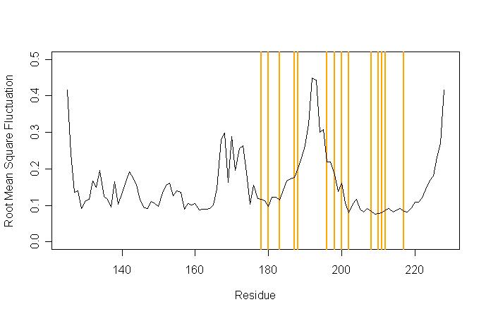
To get an impression of the relevance of these results, here is a plot of the RMSF of the human prion protein (PDB ID 1qlz), in which residues are marked for which mutations are known that cause Creutzfeld-Jakob Disease (CJD):

Now view the two pdb files, average.pdb and bfactors.pdb, by loading them into Pymol. Then color the structure bfactors.pdb according to b-factors and inspect the flexible regions. Note the average structure is an unphysical structure. Have a look at some of the side chains, and notice the effect of averaging over conformations.

pymol average.pdb bfactors.pdb

spectrum b, selection=bfactors

The colors are distributed over the range of b-factor values, with blue representing the lowest (most stable) and red the highest (most fluctuating). Although a bit off-topic, it is good to realize that, although rainbow colours seem appealing, they are hard to interpret and show transitions that are not actually present. For those reasons it is often better to use a different colour range, for instance from green through white to magenta:

spectrum b, palette=green_white_magenta, selection=bfactors

Often the range of values is notably non-linear, so that most of the structure appears in one color and only a few peripheral sites show up in another. You can adjust the colour range by truncating the maximum value, or by transforming the range, e.g., by using a logarithmic scale:

alter all, q = math.log(b) spectrum b

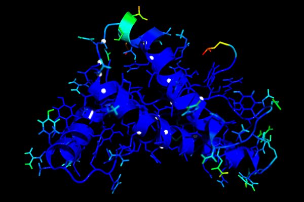
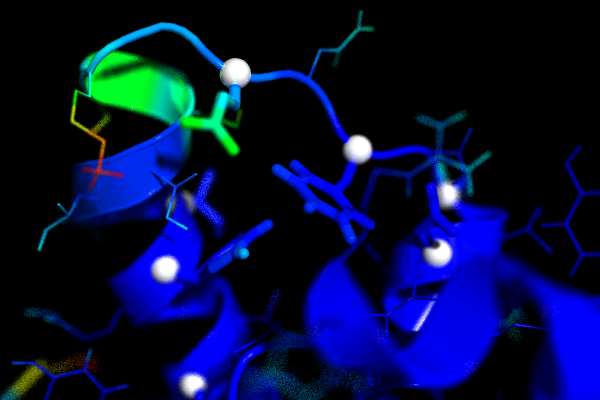
The following images shows the human prion protein (1qlz) coloured according to the b-factors calculated from a simulation. Blue is low, red is high. The white spheres mark the residues for which mutations are known that cause prion diseases. The second image shows a close up of the loop preceding the third helix. On the left side of the image you can see that the last part of the second helix has relatively high b-factors.

Convergence of RMSD

As the calculation of the RMSF also gave the average structure, we can now commence with calculating the RMSD. The RMSD is commonly used as an indicator of convergence of the structure towards an equilibrium state. As mentioned above, the RMSD is merely a distance measure and is most meaningful for low values. The RMSD is calculated using the program g_rms. First calculate the RMSD for all protein atoms, using the starting structure as a reference:

g_rms -f traj.xtc -s topol.tpr -o rmsd-all-atom-vs-start.xvg

==Q== At what time and value does the RMSD reach a plateau? ( T )

Now calculate the RMSD again, but only select the backbone atoms:

g_rms -f traj.xtc -s topol.tpr -o rmsd-backbone-vs-start.xvg

This time the RMSD settles at a lower value, which is the result of excluding the, often flexible, side chain atoms. In both cases the RMSD increases to a plateau value. This means that the structure of the protein reaches a certain distance from the reference structure and then keeps that distance more or less. However, with increasing distance, the amount of conformations available also increases. This means that, although the RMSD has reached a plateau value, the structure may still be progressing towards its equilibrium state. For this reason, it is advisable also to check the convergence towards the average structure.

echo 1 | trjconv -f traj.xtc -s topol.tpr -o protein.xtc

g_rms -f protein.xtc -s average.pdb -o rmsd-all-atom-vs-average.xvg

g_rms -f protein.xtc -s average.pdb -o rmsd-backbone-vs-average.xvg

Compare the resulting graphs to the previous ones. Note at which point the RMSD values level off.

==Q== Briefly discuss two differences between the graphs against the starting structure and against the average structure. Which is a better measure for convergence?

Convergence of radius of gyration

As a final part of the QA, we calculate the radius of gyration. This measure gives an indication of the shape of the molecule at each time. The radius of gyration compares to the experimentally obtainable hyrdodynamic radius. It can be calculated using g_gyrate. This program will also give the individual components, which correspond to the eigenvalues of the matrix of inertia. This means that the first individual component corresponds to the longest axis of the molecule, while the last corresponds to the smallest. In effect, the three axes give a global indication of the shape of the molecule. Issue the command

g_gyrate -f traj.xtc -s topol.tpr -o radius-of-gyration.xvg

Have a look at the radius of gyration and the individual components and note how each of these progress to an equilibrium value.

==Q== At what time and value does the radius of gyration converge? ( T )

Structural analysis: properties derived from configurations

At this point we have ended the first part of the analysis, involving a visual inspection and quality assurance checks. Now time has come to dig in a bit deeper and have a look at what's going on inside the proteins. This second part of the analysis covers structural properties that can be calculated from protein configurations, such as the number of hydrogen bonds and the solvent accessible surface.

When asked for a selection choose "Protein" if no selection is specifically stated or does not follow logically from the text.

Having assured that the simulation has converged to an equilibrium state, it is time to do some real analysis. Analysis of simulation data can be divided into several categories. The first category comprises of the interpretation of single configurations according to some function to obtain a value, or a number of values, for each time point. The RMSD and the radius of gyration are examples. Such properties can be called configurational, dependent or instantaneous properties. Next to that, one can analyze processes in the time domain, e.g. through averaging, as (auto)correlations or fluctutations, and across simulations. In this section, a number of common analyses will be performed, each of which yields a time series of values directly derived from the trajectory (the coordinates over time). The questions may refer to the screen output from the program or to graphs.

Solvent accessible surface area

One property which can be of interest is the surface area of the protein which is accessible to solvent, commonly referred to as the solvent accessible surface (SAS) or the solvent accessible surface area (SASA). This can be further divided into a hydrophilic SAS and a hydrophobic SAS. In addition, the SAS can be used together with some empirical parameters to obtain an estimate for the free energy of solvation. All four of these parameters are calculated by the program g_sas. This program also allows calculating the average SAS over time per residue and/or per atom. Issue the following command, specifying Protein, for the group to calculate the SAS for, as well as for the output group, and have a look at the output files.

g_sas -f traj.xtc -s topol.tpr -o solvent-accessible-surface.xvg -oa atomic-sas.xvg -or residue-sas.xvg

==Q== What are the average values for the hydrophobic and the hydrophilic SAS over the last nanosecond of the simulation? ( T )

Hydrogen bonds

Another property which can be informative is the number of hydrogen bonds, either internally (Protein - Protein) or between the protein and the surrounding solvent. The presence or not of a hydrogen bond is inferred from the distance between a donor-H - acceptor pair and the donor - H - acceptor angle. To calculate the hydrogen bonds issue the following commands, and have a look at the output files using xmgrace:

g_hbond -f traj.xtc -s topol.tpr -num hydrogen-bonds-intra-protein.xvg

g_hbond -f traj.xtc -s topol.tpr -num hydrogen-bonds-protein-water.xvg

==Q== Estimate the number of hydrogen bonds within the protein and between protein and solvent over the last nanosecond. ( T )

==Q== Discuss the relation between the number of hydrogen bonds for both cases and the fluctuations in each.

Specific hydrogen bonds can be investigated using an index file that contains the numbers of the atoms to be included. For 1qlz, the plot of the RMSF shown in the first part of the analysis showed high values for the end of helix two. It is worth inspecting the backbone hydrogen bond between residues 188 and 192. For your structure, find the residue numbers corresponding to those positions and have a look at the hydrogen bond between them. Note the atom and residue numbers may have changed during the processing, so the right numbers need to be identified. First load the structure in pymol, and overlay the human form. Then show the residue numbers, colouring those in the reference structure yellow.

pymol bfactors.pdb

fetch 1qlz, async=0
hide everything
show cartoon
show spheres
set sphere_scale, 0.25
align 1qlz, bfactors
label n. ca, resi
set label_color, yellow, 1qlz

After identifying the residues in your structure, search these residues in the file confout.gro and write down the atom numbers (third column). Then create a new file, listing two groups, according to the following format (mind changing the atom numbers):

cat <<EOF >index.ndx
[ THR188 ]
721 722 723 724 725 726 727 728 729
[ THR192 ]
756 757 758 759 760 761 762 763 764
EOF

g_hbond -f traj.xtc -s topol.tpr -num hydrogen-bonds-residues.xvg -n index.ndx

==Q== What can you say about the stability of the hydrogen bond from this graph?

Salt bridges

Besides hydrogen bonds, proteins also often form salt bridges between oppositely charged residues. These can have an important stabilizing effect on the structure of the protein, in particular when they are embedded in a hydrophobic environment, such as the core of the protein. The existence of salt bridges can be investigated with g_saltbr. When requested (through the flag -sep) this program will generate an output file for every pair of oppositely charged residues which at some point in the trajectory are within a certain cut off distance from each other (here 0.5 nm, specified through the option -t). This gives a large number of files, so it is best to make a separate directory for running this analysis. Execute the following commands:

mkdir saltbridge

cd saltbridge

g_saltbr -f ../traj.xtc -s ../topol.tpr -t 0.5 -sep

Just to make things a bit clearer, remove the files involving sodium and chloride ions:

rm *CL* *NA* \#*

Find the residue numbers in your structure corresponding to Arginine 156 and Aspartate 196 in the reference structure (1QLZ, check the procedure described above), and look at the graph showing the interaction between them.

==Q== What can you say about the interactions? The acidic residue is highly conserved and mutation of that aspartate in humans is known to result in prion disease. What could be the cause of that?

Secondary structure

Among the most common parameters to judge protein structure is the assignment of secondary structure elements, such as α-helices and β-sheets. One such assignment is provided by dssp. This program, which is not part of the gromacs distribution, but can be obtained at the CMBI, Radboud University. Gromacs does provide an interface to dssp, to allow the calculation of secondary structure for each frame of a trajectory. To use this, first set an environment variable DSSP, which points to the location of the program. Then run do_dssp as follows:

export DSSP=/home/student/Desktop/dssp

do_dssp -f traj.xtc -s topol.tpr -o secondary-structure.xpm -sc secondary-structure.xvg -dt 10

The file secondary-structure.xvg contains a time series, listing the numbers of residues associated with each type of secondary structure per frame. More detailed information is in the .xpm file, which gives a color coded assignment of the secondary structure per residue over time. The .xpm file can be viewed with e.g. the Gimp, but some useful metadata can be added with the gromacs tool xpm2ps and the result can be viewed with gview or a similar program.

xpm2ps -f secondary-structure.xpm -o secondary-structure.eps

gv secondary-structure.eps

==Q== Discuss some of the changes in the secondary structure, if any.

==Q== The results so far probably indicates that part of the second helix is unstable. Compare the stability of this part of the secondary structure in your protein with that of others.

Ramachandran (phi/psi) plots

The phi and psi torsion angles of the protein backbone are two parameters that are useful to gain insight into the structural properties of a protein. The plot of phi against psi is called a Ramachandran plot and certain regions of this plot are characteristic of secondary structure elements or of amino acids. Other regions are considered forbidden (inaccessible). Projection of the phi/psi angles over time may give insight in structural transitions. These angles can be calculated by the program g_rama, albeit in a bit of a crude way, namely put all together in a single file. To investigate single residues, the linux progam 'grep' can be used to select them out of the plot.

g_rama -f traj.xtc -s topol.tpr -o ramachandran.xvg

This file contains all phi/psi angles for all residues. To extract the angles for a single residue, e.g. GLU-200 (glutamate), type:

grep GLU-200 ramachandran.xvg | awk '{print $1 " " $2'} > rama-GLU-200.xvg

Do this to extract the ramachandran plots for the residues corresponding to Glutamate 200 and Aspartate 202, and view them using xmgrace. In the structures deposited in the PDB these residues were classified helical.

==Q== What can you say about the conformation of these residues, based on the ramachandran plots (see the image given above)?

Analysis of dynamics and time-averaged properties

Root mean square deviations again

The root mean square deviation (RMSD) was already calculated to check the convergence of the simulation. But it can also be used for further analysis. The RMSD is a measure relating two structures. If we calculate the RMSD for each combination of structures in a trajectory file, then we can see if there are groups of structures belonging together, sharing structural features. Such structures will have lower RMSD values within the group and higher RMSD values with other structures. Representing the RMSD values in a matrix, this also allows identifying transitions.

To build an RMSD matrix, g_rms is called with two trajectories. In our case, the same trajectory will be used for both. We will only take every second frame in the trajectory file, giving a 1001x1001 matrix. Select the protein.

g_rms -s topol.tpr -f traj.xtc -f2 traj.xtc -m rmsd-matrix.xpm -dt 10

The resulting matrix is in grayscale. To make it more clear download the script xpm2ppm.py and use it to map a color gradient to the image. Then view the image.

xpm2ppm.py -f rmsd-matrix.xpm -o rmsd-matrix.ppm

display rmsd-matrix.ppm

View the file rmsd-matrix.ppm. How many transitions can you distinguish?

Cluster analysis

On the basis of the distances between structures, the RMSD, the these can also be assigned to a set of clusters that reflects the range of conformations accessible and the relative weight of each of these. This can be done using a clustering algorithm, of which several are implemented in g_cluster. This program generates a number of output files. Check the programs help file to see what each means. Then run the program. Note that we already calculated the RMSD matrix and can use it as input to g_cluster.

g_cluster -h

g_cluster -s topol.tpr -f traj.xtc -dm rmsd-matrix.xpm -dist rmsd-distribution.xvg -o clusters.xpm -sz cluster-sizes.xvg -tr cluster-transitions.xpm -ntr cluster-transitions.xvg -clid cluster-id-over-time.xvg -cl clusters.pdb -cutoff 0.25 -method gromos -dt 10

==Q== How many clusters were found and what were the sizes of the largest two? ( T )

Open the file clusters.pdb with pymol and compare the structures from the first two clusters.

disable all
split_states clusters
delete clusters
for i in range(3,100): cmd.delete( "clusters_%04d" %i )
dss
show cartoon
util.cbam clusters_0002
align clusters_0001 and ss h, clusters_0002 and ss h

==Q== What are the most notable differences between the two structures?

Distance RMSD

One drawback of using the RMSD for comparing structures is that it involves least squares fitting, which will influence the results. But the structure of a protein can also be represented by the set of interatomic distances. These can be used to obtain a measure of comparison that does not depend on fitting: the distance RMSD (dRMSD). This can be obtained using the program g_rmsdist.

g_rmsdist -s topol.tpr -f traj.xtc -o distance-rmsd.xvg

==Q== At what time and value does the dRMSD converge and how does this graph compare to the standard RMSD?

Analysis of interatomic distances, NOE's from simulations

The program g_rmsdist used above can also be used for further distance analysis. In particular, it may be useful to look at the mean distances between atoms and the fluctuations in these distances to get an idea of the structure and stability. Calculate the matrices containing the mean distances and distance fluctuations for each pair of atoms in the protein. Recolor the images using the procedure given above and display the resulting .ppm files (rmsmean.ppm and rmsdist.ppm).

g_rmsdist -s topol.tpr -f traj.xtc -rms rmsdist.xpm -mean rmsmean.xpm -dt 10

==Q== Briefly explain the images: rmsmean in terms of structure and rmsdist in terms of flexibility/stability. Recall the information from earlier analysis and viewing the structure

These distances are also important from an experimental point of view. Bounds on distances between atoms can be derived from NMR experiments, exploiting the Nuclear Overhauser Effect (NOE), and are the main driving force between NMR structure calculations. The NOE signals that should be expected for a protein if the model is correct, can be calculated from a MD simulation. These are intimately linked to the distances, in particular to the r^-3 and r^-6 weighted distances. These can also be calculated using g_rmsdist.

g_rmsdist -s topol.tpr -f traj.xtc -nmr3 nmr3.xpm -nmr6 nmr6.xpm -noe noe.dat -dt 10

Recolor nmr3.xpm and nmr6.xpm and have a look at these matrices. Also view the file noe.dat.

==Q== What are the smallest 1/r^3 and 1/r^6 averaged distances in the simulation? ( T )

Relaxation and order parameters

The relaxation of a vector is calculated as its autocorrelation. For proteins, this usually involves the backbone N-H or side chain C-H vectors. The autocorrelation gives a measure of how long a vector will keep its direction, thus providing an indication of flexibility or stability. The order parameter is the long term limit of the autocorrelation. If a molecule is free to rotate, the order parameter inevitably decreases to zero, but in the frame of a molecule (internal reference frame), the order parameter will usually have a distinct value, reflecting the overall stability. By fitting the protein, the reference frame can be fixed and the order parameter can be determined.

N-H order parameters can be calculated using g_chi. This program can write a .pdb file in which the order parameter is added to the b-factor field, allowing easy visualization. The program also calculates J-couplings that can be compared to results from NMR or used as basis for NMR experiments.

g_chi -s topol.tpr -f traj.xtc -o order-parameters.xvg -p order-parameters.pdb -jc Jcoupling.xvg

Have a look at the order parameters in the .xvg file and look at the .pdb file with Pymol, colouring the residues according to the values in the b-factor field.

==Q== Write down the start and end residues, and the average value for the two regions having highest order parameters. ( T )

==Q== How do the order parameters compare to the fluctuations (RMSF)?

Configurational principal component analysis

See Leach Chapter 9.14 for more information on the following section.

An often used, but often little understood, method of analysis is principal component analysis (PCA) of the trajectory. This method, which is sometimes also referred to as 'essential dynamics' (ED), aims at identifying large scale collective motions of atoms and thus reveal the structures underlying the atomic fluctuations. The fluctuations of particles in a molecular dynamics simulation are by definition correlated due to interactions between the particles. The degree of correlation will vary and notably particles which are directly connected through bonds or lie in the vicinity of each other will move in a concerted manner. The correlations between the motions of the particles give rise to structure in the total fluctuations in the system and for a macromolecule this structure is often directly related to its function or (bio)physical properties. Thus, the study of the structure of the atomic fluctuations can give valuable insight in the behaviour of such macromolecules. However, it does require a certain level of understanding of linear algebra methods and multivariate statistics to interpret the results and identify the shortcomings of the method. In particular, the aim of principal component analysis is to describe the original data in terms of new variables which are linear combinations of the original ones. This is also the most important problem with PCA: it only offers an interpretation in terms of linear relationships between atomic motions.

The first step in PCA is the construction of the covariance matrix, which captures the degree of collinearity of atomic motions for each pair of atoms. The covariance matrix is, by definition, a symmetric matrix. This matrix is subsequently diagonalized, yielding a matrix of eigenvectors and a diagonal matrix of eigenvalues. Each of the eigenvectors describes a collective motion of particles, where the values of the vector indicate how much the corresponding atom participates in the motion. The associated eigenvalue gives equals the sum of the fluctuation described by the collective motion per atom, and thus is a measure for the total motility associated with an eigenvector. Usually most of the motion in the system (>90%) is described by less than 10 eigenvectors or principal components.

The covariance analysis may give a substantial number of files. For that reason it is better performed in a subdirectory:

mkdir COVAR

cd COVAR

The construction and diagonalization of the covariance matrix can be performed with the program g_covar. Issue the following command to perform the analysis. Note that the construction and diagonalization of a covariance matrix may take some time.

g_covar -s ../topol.tpr -f ../traj.xtc -o eigenvalues.xvg -v eigenvectors.trr -xpma covar.xpm

==Q== What are the dimensions of the covariance matrix and what is the sum of the eigenvalues? ( T )

The sum of the eigenvalues is a measure of the total motility in the system. It can be used to compare the flexibility of a protein under different conditions, but it is hard to give a meaningful interpretation when comparing proteins of different sizes.

Now have a look at the covariance matrix itself, stored in covar.xpm.

xview covar.xpm

The matrix shows the covariances between atoms. Red means that two atoms move together, whereas blue means they move opposite to each other. The diagonal corresponds to the RMSF plot obtained earlier, with the intensity of the red color indicating the amplitude of the fluctuations.

==Q== Look at the two most moving parts, excluding the termini. How do they move with respect to each other and to the rest of the protein?

From the covariance matrix you can see that groups of atoms move in a correlated or anti-correlated manner. This allows rewriting the total motion into collective motions of groups of atoms. As mentioned, the eigenvalues, stored in the file eigenvalues.xvg, indicate the total fluctuation explained by the corresponding eigenvector.

==Q== Look at the file eigenvalues.xvg with a text editor. Calculate the percentage and cumulative percentage of the motion explained for the first five eigenvectors. ( T )

The first five eigenvectors would typically capture the main motions, accounting for >80% of the total motility. If the total fluctuation explained is lower, that suggests that there are no clear-cut collective motions.

To see what these eigenvectors actually mean, further analysis can be performed with the tool g_anaeig. To have a closer look at the first two eigenvectors issue the following commands:

g_anaeig -s ../topol.tpr -f ../traj.xtc -v eigenvectors.trr -eig eigenvalues.xvg -proj proj-ev1.xvg -extr ev1.pdb -rmsf rmsf-ev1.xvg -first 1 -last 1

g_anaeig -s ../topol.tpr -f ../traj.xtc -v eigenvectors.trr -eig eigenvalues.xvg -proj proj-ev2.xvg -extr ev2.pdb -rmsf rmsf-ev2.xvg -first 2 -last 2

The eigenvectors correspond to directions of motion. The option -extr extracts the extreme structures along the selected eigenvectors from the trajectory. Have a look at these structures by loading them into PyMOL:

pymol ev?.pdb

Split the models in the pdb files and delete the originals.

split_states ev1

split_states ev2

delete ev1 or ev2

Colour the models. This will result in the extreme structures from eigenvector 1 to be displayed in blue-green and those from eigenvector two in yellow-red. Then display them in cartoon representation.

spectrum count

dss

hide everything

show cartoon

Using PyMOLs 'align' command, you can draw bars indicating the differences between two conformations.

align ev1_0001 and (n. c,n,ca),ev1_0002 and (n. c,n,ca),object=diff1

align ev2_0001 and (n. c,n,ca),ev2_0002 and (n. c,n,ca),object=diff2

==Q== What is the largest difference between the extreme structures for eigenvector 1? And for eigenvector 2?

To understand the meaning of these eigenvectors, imagine what would happen if we explain motions of a salesperson between European cities in this way. These motions can be explained within the coordinate system of the Earth, in which case we need to consider three coordinates at each position. Although correct, it is not optimal if you only want to explain the motions of the salesperson. Since in principle any coordinate system is as good as any other, we can define a new one, to best explain the motions of the salesperson. In fact, since the surface of the Earth can locally be represented two-dimensionally, we only need two coordinates, rather than three. Intuitively, one would argue for south-north and west-east axes. But one can also infer the axes from the motions. Let's say the salesperson travels most on the axis London-Athens. That axis would then be the first eigenvector. The second eigenvector would be taken orthogonal to the first. In this way, each position of the salesman in Europe would be uniquely defined by the projections onto these two eigenvectors. Plotting the projections against each other would show the path travelled. The extreme projections along the first eigenvector could correspond to Reykjavik and Moscow, even though these do not actually lie on the axis.

For protein conformations it is exactly the same. The extreme projections you have looked at do not need to correspond to physical structures, but they allow to visualize the motion along the axis and the total extent of the motion. To get an idea of the travels of the protein through conformational space, we can plot the projections on eigenvector 2 against those on eigenvector 1. To do so, we extract the projections from both .xvg files and combine them in the file ev1-vs-ev2.dat. Note that the character '>' indicates the redirection of output from the screen to a file, so that you won't see any output.

grep -v "^[#@]" proj-ev1.xvg | awk '{print $2}' > proj-ev11.dat

grep -v "^[#@]" proj-ev2.xvg | awk '{print $2}' > proj-ev12.dat

paste proj-ev11.dat proj-ev12.dat > ev1-vs-ev2.dat

To illustrate the progress of the simulations, we also extract the projections for the last 7.5 ns (the last 1500 points) and the last 5.0 ns (the last 1000 points). Then we load it into xmgrace.

tail -1500 ev1-vs-ev2.dat > last-7.5ns.dat

tail -1000 ev1-vs-ev2.dat > last-5.0ns.dat

xmgrace ev1-vs-ev2.dat last-7.5ns.dat last-5.0ns.dat

==Q== What is the shape of the projections? Are these mutually independent (oval distribution)?

==Q== Would the same eigenvectors (axes) be obtained if the analysis were performed on the last 7.5 ns? And on the last 5.0 ns?

The end

Write a concluding paragraph, comparing the results obtained for the different proteins. Note that the residues selected for calculating specific hydrogen bonds and for calculating the ramachandran plots were chosen to correspond between the different proteins. Also reflect on the overall stability and the probability that the structure deposited in the PDB properly reflects the solution structure. In other words, does the structure stay close to the starting structure or does it drift away and how much?

Thank you for following this tutorial, even if some of you were made to do so. I would welcome any feedback to improve it. For the students following the course Molecular Modeling and Mathematics, please add suggestions at the end of the report. You won't be negatively judged for it :) Others may send comments to tsjerkw -any human will know how to replace this for an at- gmail, obviously followed by dot com.

Quick Links

• Introduction
• Starting structures
• Simulation
• Analysis
• Report