


Physisorption on particle-based surfaces
- Details
- Last Updated: Thursday, 21 November 2019 15:04
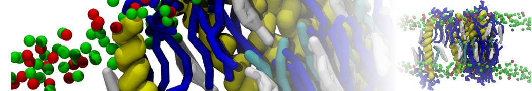
Self-assembly of functionalized alkanes on a graphite surface
This tutorial guides you on how to perform self-assembly simulations on a graphite flake using a special version of the coarse-grained force-field MARTINI [1], similar to work done in publication [2]. The Martini force-field was originally developed for lipids [1] and then extended to many other systems including self-assembly on a graphite flake [2,3]. For learning purposes, we will limit ourselves to a tiny graphite flake with a small number of adsorbent molecules. Such simulations can be done on a personal computer within 2h. The tutorial is prepared for GROMACS 2016 versions and may need (small) changes in other versions. All files for this tutorial can be found in this zip file.
The aim of the tutorial is two-fold:
- it contains specific information to set up the self-assembly simulations of long-chain functionalized molecules on graphite
- it contains a method to construct a regularly packed surface consisting of a number of layers of beads: this method can be used to construct any such surface or crystal regardless of the nature of the beads or application
This tutorial assumes a basic knowledge of the Linux operating system and some experience with gromacs. It is helpful to have a basic understanding of the gromacs molecular dynamics package and the Martini force-field. You can find tutorials on these topics at http://cgmartini.nl and http://www.mdtutorials.com/gmx/lysozyme/index.html.
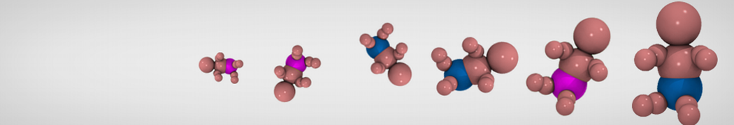
In this tutorial, we will perform a simple simulation of self-assembly (that is adsorption and rearrangement) on a graphite surface from a random configuration of adsorbent in a solvent. We will study here self-assembly of a linear functionalized alkane, AM25, which consist of 6 beads (two P1 polar and four C1 apolar beads, respectively, arranged as C1-P1-C1-C1-P1-C1), which can represent N,N′-decanomethylenebispentamide (C4H9-CO-NH-(CH2)10-NH-CO-C4H9). For more information, look into publication [2]. As a solvent, we use phenyloctane, which in its coarse-grained representation consist of 5 beads (three SC4 beads in a ring and two C1 beads in a tail)
0. Setting up the system
Download the zip file, and unzip it. It expands to a directory or folder called Tutorial. Go into the folder of the tutorial. For purposes of this tutorial this will be our working directory:
$ cd Tutorial
Make an empty directory in which you will test the simulation protocol:
$ mkdir testSA
$ cd testSA
First copy a sample topology file:
$ cp ../topology/sample_topol.top topol.top
The topology file consist of references to parameters of force-fields and number of molecules in the system. Here is the sample_topol.top file:
#include "../FF/martini_v2.15.itp"
#include "../FF/martini_v2.0_solvents.itp"
#include "../FF/martini_v2.0_graphite.itp"
#include "../FF/martini_v2.0_graphite.itp""
[ system ]
Adsorption on graphite
[ molecules ]
GRAP 1600
AM25 50
PHEO 300
The first four lines describe where parameters of force-field can be found (in subdirectory "Tutorial/FF"), then there is [ system ] with a title of simulation, and then [ molecules ], after which there are types and numbers of molecules of each type used in the simulation. For this tutorial, we use 1600 beads of graphite, 50 molecules of AM25, and 300 molecules of solvent PHEO. The subfolder "Tutorial/topology" also contains other topologies used in publication [2].
Copy the coordinate file of a small graphite flake from the "Tutorial/gro" folder (to learn how to make a graphite flake yourself look at the end of this tutorial page). This box contains 1600 graphite beads in four layers, arranged in a hexagonal pattern. The beads are located inside the box, making sure there is space between the periodic images in all directions. This is why it is called a "flake", as opposed to a "surface". In many modeling applications, surfaces (of solids) are modeled as periodic entities, with a number of unit cells explicitly described and connected across the periodic boundaries. Here, this is NOT the case.
$ cp ../gro/small_graphite.gro 0_box.gro
Insert adsorbent molecules into this box using the "gmx insert-molecules" command: the coordinate file for single molecules of adsorbents are in the "Tutorial/gro" subdirectory. Here, we insert 50 adsorbent molecules of the AM25 kind:
$ gmx insert-molecules -f 0_box.gro -ci ../gro/AM25.gro -o 0_box_ad.gro -nmol 50
Add solvent molecules using the "gmx solvate" command: here we use the -maxsol option to limit the number of molecules to 300 (however, you don't have to use it, but you have to then make an appropriate change of the number of molecules in topol.top file):
$ gmx solvate -cp 0_box_ad.gro -cs ../gro/phenyloctane.gro -o 0_box_sol.gro -p topol.top -maxsol 300
The subfolder "pictures" includes snapshots of different stages of the processes filling the box.
Now it is time to perform simulations with the system prepared.
1. Energy minimization
After our system is set up, perform energy minimization, to remove all bad contacts (which could result in numerical instability and an explosion of the system). All parameter files for the simulation engine are in the "Tutorial/mdp" folder. All *.mdp files are similar to one present on other tutorials of Martini except lines in which we specify that graphite beads are frozen (freezegrps = GRAP and freezedim= Y Y Y). The graphite beads do not move during the course of simulation (but they do interact with adsorbent and solvent molecules). This is a choice that is usually made to limit the computational effort. The graphite surface when run without the "freezegrps" option is stable at small time-steps, but defects might occur over time.
$ gmx grompp -f ../mdp/1_em.mdp -c 0_box_sol.gro -p topol.top -o 1_em.tpr
[
Note that you may have to ignore WARNINGS. This can be done by adding the -maxwarn option to the gmx grompp command, e.g. if you need to ignore 1 warning:
$ gmx grompp -f ../mdp/1_em.mdp -c 0_box_sol.gro -p topol.top -o 1_em.tpr -maxwarn 1
]
$ gmx mdrun -v -deffnm 1_em
[
Note that here you may have to limit the number of threads because the system is quite small, and may be too small for the domain decomposition over the available number of nodes. To use 4 threads, for example:
$ gmx mdrun -v -deffnm 1_em -nt 4
]
Energy minimization will produce an local energy minimized structure in the 1_em.gro file, which we use for further simulations.
2.Equilibration
We perform the equilibration in two stages: first we equilibrate at constant volume and temperature (NVT ensemble) and then at constant pressure and temperature (NPT ensemble).
Equilibrate the system in the NVT ensemble:
$ gmx grompp -f ../mdp/2_nvt.mdp -c 1_em.gro -p topol.top -o 2_nvt.tpr -maxwarn 1
$ gmx mdrun -v -deffnm 2_nvt
We use the option "-maxwarn 1" to ignore one warning:
WARNING 1 [file ../mdp/2_nvt.mdp]:
For proper integration of the Berendsen thermostat, tau-t (0.3) should be at least 5 times larger than nsttcouple*dt (0.3)
which we ignore because we are performing this step to get a reasonable starting structure for production simulations and are not too concerned that the statistical ensemble or integration is not exact.
Equilibrate system in the NPT ensemble:
$ gmx grompp -f mdp/2_npt.mdp -c 2_nvt.gro -p topol.top -o 2_npt.tpr -maxwarn 2
$ gmx mdrun -v -deffnm 2_npt
In this case, we use "-maxwarn 2" to ignore two warnings:
WARNING 1 [file ../mdp/2_npt.mdp, line 65]:
All off-diagonal reference pressures are non-zero. Are you sure you want to apply threefold shear stress?
We ignore it because we want to allow deformations of the box only in the z-direction (the direction perpendicular to the plane of the graphite flake. The flake should not come near its periodic image, and therefore the lateral (x, y) directions are kept fixed.
WARNING 2 [file ../mdp/2_npt.mdp]:
For proper integration of the Berendsen thermostat, tau-t (0.3) should be at least 5 times larger than nsttcouple*dt (0.3)
3. Run simulation
After the temperature and pressure of the system are equilibrated, it is a time to perform a production simulation:
$ gmx grompp -f ../mdp/3_run.mdp -c 2_npt.gro -p topol.top -o 3_run.tpr -maxwarn 2
$ gmx mdrun -v -deffnm 3_run
This command will produce several files, from which final structure is in 3_run.gro and trajectory in 3_run.xtc file. Such a simulation on a PC (CPU Intel(R) Core(TM) i7-5600U CPU @ 2.60GHz) takes about 2h.
You can visualize this trajectory and structure using visualization program such as VMD (http://www.ks.uiuc.edu/Research/vmd/). A quick impression of the system can be gotten with "gmx view" if you have installed it (not standard!):
$ gmx view -s 3_run.tpr -f 3_run.xtc
Select which molecules you want to see, and find the "Display/Animate" tab to click through the trajectory. If you are happy, you can spend more time on better visualization, for example using VMD. It is recommended that you first convert your trajectory, (1) to avoid long bonds appearing between beads that are on the other side of the periodic box ("-pbc whole"), and (2) to make VMD draw bonds between beads that have much longer bond-lengths than the standard cut-off of VMD ("-o 3_run.tng"; the .tng format knows which bonds to draw and makes the plug-in "cg_bonds.tcl" largely obsolete).
$ gmx trjconv -f 3_run.xtc -pbc whole -o 3_run.tng
$ vmd 3_run.tng
This concludes the tutorial on the set-up of a small system for 2D self-assembly on graphite from solution. In this tutorial, you were given a small graphite flake in a simulation box. Here is how you can make your own!
4. Custom size of graphite flake:
NOTE that the following procedure can be used to create any regular arrangement of beads given a unit cell!
In the main directory Tutorial, make a new folder for testing:
$ mkdir testFlakeSetup
$ cd testFlakeSetup
You can make a custom size of the graphite flake from the unit cell given in the "Tutorial/gro" subfolder file "cell.gro"; this cell contains just two beads from which a graphite flake can be produced using the command:
$ gmx genconf -f ../gro/cell.gro -nbox 20 20 2 -o 0_out.gro
This creates rhombic graphite flake of 20x20 unit cells in the x- and y-directions and two unit cells (four layers) in the z direction (the cell contains two beads in the z-direction). Subfolder "Tutorial/gro" also contains a coordinate file (graphite_paper.gro) of the graphite flake used in publication [2].
Next, create a simulation box with a given size:
$ gmx editconf -f 0_out.gro -o 0_box.gro -box 7 7 7 -angles 90 90 60
The "-angles" option causes the simulation box to be hexagonally shaped in the x-y dimension (as is the flake), and with right angles to the z-direction. It is essential that the simulation box is larger than the graphite flake (the periodically connected graphite surface causes packing artefacts).
Having created your own box, you can use it to fill with adsorbents and solvent, or do other cool things you might think of...
5. Simulation of other molecules:
Since some of the parameters for simulation engine reference to a specific group of molecules, to simulate different molecules, you need to make appropriate changes in mdp files. For example, if you would like to simulate AL1 molecules, you can do it using one simple command. You may want to keep the existing mdp files, so...
In the main directory Tutorial, make a new folder for testing:
$ cp -R mdp mdp-AL1
$ sed -i 's/AM25/AL1/g' mdp-AL1/*mdp
which changes all the names of molecules AM25 to AL1 in mdp files.
The coordinate files for the different adsorbents are in "Tutorial/gro" subfolder.
References:
[1] Marrink, S. J., Risselada, H. J., Yefimov, S., Tieleman, D. P., and De Vries, A. H. (2007) The MARTINI force field: coarse grained model for biomolecular simulations. J. Phys. Chem. B 111, 7812–7824.
[2] Piskorz, T. K., Gobbo, C., Marrink, S.-J., Feyter, S. de, Vries, A. H. de, Esch, J. H. van (2019). Nucleation mechanisms of self-assembled physisorbed monolayers on graphite. J. Phys. Chem. C, 123, 17510-17520.
[3] Gobbo, C., Beurroies, I., De Ridder, D., Eelkema, R., Marrink, S. J., De Feyter, S., De Vries, A. H. (2013). MARTINI model for physisorption of organic molecules on graphite. Journal of Physical Chemistry C, 117(30), 15623-15631.
Tutorial contributed by Tomasz K. Piskorz.