Molecular Modeling Practical
This tutorial introduces the student to the practice of Molecular Dynamics (MD) simulations of proteins. The protocol used is a suitable starting point for investigation of proteins, provided that the system does not contain non-standard groups. At the end of the tutorial, the student should know the steps involved in setting up and running a simulation, including some reflection on the choices made at different stages. Besides, the student should know how to perform quality assurance checks on the simulation results and have a feel for methods of analysis to retrieve information.
Introduction and Outline
The aim of this tutorial is to investigate differences in the conformation and dynamics of a human ubiquitin-conjugating enzyme (E2). At the end of the tutorial the student should be able to:
- Set up and run Molecular Dynamics Simulations of proteins using Gromacs
- Perform quality assurance checks and analysis on simulation results
- Compare simulation results obtained from different simulations
- Derive some theoretical knowledge about these enzymes and their potential interaction profile with the Ubiquitin-Ligase proteins
Commands are given in white on a blue background. These have to be typed carefully, since the shell (the program parsing the commands) is case-sensitive. A common error that may occur is replacing a 0 (digit zero) for an O (capital letter O), an l (lower case letter l) for a 1 (digit one), or vice-versa. You might want to copy-paste the commands, which is as simple as selecting them with the mouse and pressing the middle mouse button on the spot where the command should be entered. Now first try the following commands:
whoami
This lists your current user name. Make sure you're not logged in as "root".
ls -l
This gives a listing of the things that are in the directory where you are. Use this if you encounter errors like "file not found".
pwd
This command shows you the full path of the directory where you are.
Mind that copy-pasting does not relief you from reading the text! You can't run the tutorial without the instructions around the commands. It is naively assumed that the intention of the one following the tutorial is to learn something. In some cases you might be reminded to read carefully, by a comment like the following:
Read carefully!
Ubiquitin-Conjugating Enzymes
 Ubiquitin-Conjugating enzymes, also known as E2 enzymes,
perform the second step in the ubiquitination pathway. This reaction refers to the post-translational modification of a
protein by the covalent attachment of one or more ubiquitin monomers. The most prominent function of ubiquitin is
labeling proteins for proteasomal degradation. Besides this function, ubiquitination also controls the stability,
function, and intracellular trafficking of a wide variety of proteins.
Ubiquitin-Conjugating enzymes, also known as E2 enzymes,
perform the second step in the ubiquitination pathway. This reaction refers to the post-translational modification of a
protein by the covalent attachment of one or more ubiquitin monomers. The most prominent function of ubiquitin is
labeling proteins for proteasomal degradation. Besides this function, ubiquitination also controls the stability,
function, and intracellular trafficking of a wide variety of proteins.
Ubiquitination is an ATP-dependent process that involves the action of at least three enzymes: a ubiquitin-activating enzyme (E1), a ubiquitin-conjugating enzyme (E2), and a ubiquitin ligase (E3), which work sequentially in a cascade. Mutations linked to this pathway can cause human diseases like cancer, Parkinson's and cardiovascular diseases. The transfer of the ubiquitin tag to a substrate is highly specific, and relies mainly on the E2-E3 interactions.
Analysis of the human genome reveals the presence of 37 functional E2s and more than 700 E3 enzymes This E3 abundance implies that a single E2 must interact with multiple E3s. The family of ubiquitin-conjugating enzymes is characterized by the presence of a highly conserved ubiquitin conjugated (UBC) domain. The interaction surface with the E3 recognition domains involves three structural elements (namely helix1, loop1 and loop2).
We propose here to investigate the dynamics of a wild-type E2 protein (with the future intent of comparing to a mutant).
Molecular Dynamics
Classical molecular dynamics simulations use Newton's equations of motion to calculate trajectories of particles, starting from a defined configuration. For each particle in the system, the total force acting on it is calculated from the interactions with other particles, as described by the force field. The force divided by the mass of the particle gives the acceleration, which, together with the prior position and velocity, determines what the new position will be after a small time step. The high spatial and temporal resolution make molecular dynamics simulations useful for testing models based on experimental data, for understanding principles underlying the function and to formulate new hypotheses. Unfortunately, system sizes are limited, as are time scales.
Gromacs
This tutorial uses Gromacs
(http://www.gromacs.org/) for
performing and analysing molecular dynamics simulations. Gromacs is a
suite of programs which is freely available under the GNU GPL (General
Public License). The programs have a command-line interface, which
means that each step involves typing the name of the program and a
number of arguments. Note that the commands are case sensitive and
each command has to be typed exactly as in the tutorial. More information
about Gromacs as well as the manual can be found on the web site.
 and therefore increase its performance. Laptops won't benefit from MPI since Gromacs4.5.X now scales up to N-cores in the same machine automatically.")
Linux
Since the programs have a command-line interface, there is no escape from using a terminal. Although it is possible to run Gromacs under Windows in a terminal, there are several benefits attached to using Linux, which is the choice for this tutorial. For some students the transfer to Linux from Windows will form an obstacle as they are much used to the interface Windows offers. It is important to note that Linux is not intended to be a free clone of Windows. It is a powerful, highly costumizable operating system, which allows one to get much more performance from a computer. The transfer from Windows to Linux is sometimes described as switching from a motorcycle to a car. To start using the Linux terminal, it is necessary to know the most basic commands (ls,cd,mkdir,cp,mv,rm,more). Some more information about linux/unix can be found here and here.
Starting structures and visualization
Before anything else, starting structures have to be obtained. These can
be retrieved from the Protein
Databank, which is a repository for three dimensional structures of
proteins.
To start the tutorial, download the
structures with ID's
1y6l,
3bzh,
from the database.
All the students in a group must download these starting structures and compare them.
Check whether the downloaded structure is in fact a ubiquitin-conjugating protein; Don't mistake 1y6l for 1y61!
For each structure, find the method used to solve the structure and its resolution.
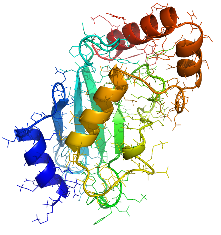
Now first have a look at the structure in a molecular viewer. The following instructions are for Pymol, which should be available on your machine. Load the structures in Pymol using
pymol *.pdb
Now Pymol should start and a window should appear showing the structures in line representation. The models are listed on the right side of the main window and can be removed from view by clicking on the name. Next to each model name are menus which allow changing the representation. Try to show the structures as cartoons and color each chain with rainbow colors from N- to C-terminus. For those inclined to use a keyboard, which is strongly encouraged, the above can also be achieved by typing in the window:
disable 1Y6L
enable 1Y6L
hide everything, all
show cartoon, all
spectrum count, rainbow, 1Y6L
To get a better view of the structural homology, fit 1Y6L onto 3BZH. This can be done using the command 'align':
align 1Y6L, 3BZH
zoom 3BZH
Note the similarities and dissimilarities between the different models. To see the differences better, it may be necessary to give each model a separate color again. Try zooming in on regions which are different and look at specific residues. You can change the representation of parts of a molecule by right-clicking on the chain. If you like the image you have, you can further improve it by typing 'ray' and save the resulting picture using 'png filename' to have a lasting memory of this tutorial.
Why is 1Y6L so much larger than 3BZH?
Now exit Pymol using the command 'quit'. As you may have noticed, all the
information necessary to draw the structures is in the respective .pdb
files. Have a look at the file using the command 'less' and try to understand
the file format. (In 'less' the space bar and 'b' scroll forward and backward
respectively, and with 'g' and 'G', you can go all the way to the top or to the end.)
The PDB file contains a lot of information regarding the protein,
the experimental methods used to determine it, conditions, etc. It also contains a listing of
each atom with the Cartesian coordinates. Note that there is no information in
the file regarding bonding, whereas Pymol, as most molecular viewers do, did
draw bonds between atoms. These bonds were inferred from the interatomic distances.
Preparation
A simplified version of the 1Y6L pdb file is waiting for you as E2Bwt.pdb.
What are the differences between the original PDB file (1Y6L) and E2Bwt?
Now it's time to start with the real Molecular Dynamics part. Remember to fill in the right filenames at every stage. In particular, the tutorial simply refers to "protein.pdb" and "protein-EM-solvated.gro", as generic names, which should be replaced with names specific to your protein (e.g. "E2Bwt.pdb" and "E2Bwt-EM-solvated.gro").
HINT: Rename your protein "protein.pdb" and you can simply copy-paste all commands.
Be sure to read carefully and to check at each step whether it was successful. Read the output! In case a program gives an error message, it is usually self-explanatory. Check file formats and program output to understand the processes at each step. Most of the files are readable, except for files ending in .tpr, .xtc, .trr and .edr.
If you feel ready, click here to proceed.