General Purpose Coarse-Grained Force Field

Topologies

Details

Last Updated: Friday, 19 August 2016 13:12

How do I create a topology for a new molecule?

Here we present a simple three-step recipe, or guide, how to proceed in parameterizing new molecules using the CG Martini model:The first step consists of mapping the chemical structure to the CG representation, the second step is the selection of appropriate bonded terms, and the third step is the optimization of the model by comparing to AA level simulations and/or experimental data. See also the Tutorial pages for guidance.

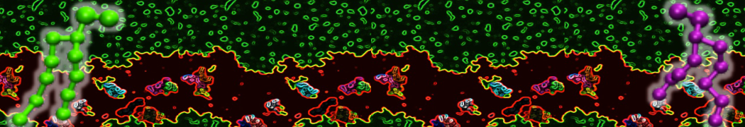
Step I, mapping onto CG representation: The first step consists of dividing the molecule into small chemical building blocks, ideally of four heavy atoms each. The mapping of CG particle types to chemical building blocks, which are presented in Table III of ref [1], subsequently serves as a guide towards the assignment of CG particle types. Because most molecules cannot be entirely mapped onto groups of four heavy atoms, some groups will represent a smaller or larger number of atoms. In fact, there is no reason to map on to an integer number of atoms, e.g. a pentadecane mapped onto four C1 particles implies that each CG bead represents 3¾ methyl(ene) groups. In case of more substantial deviations from the standard mapping scheme, small adjustments can be made to the standard assignment. For instance, a group of three methyl(ene)s is more accurately modeled by a C2 particle (propane) than the standard C1 particle for saturated alkanes. The same effect is illustrated by the alcohols: whereas the standard alcohol group is modeled by a P1 particle (propanol), a group representing one less carbon is more polar (P2, ethanol) whereas adding a carbon has the opposite effect (Nda, butanol). Similar strategies can be used for modulation of other building blocks. To model compounds containing rings, a more fine grained mapping procedure can be used. In those cases, the special class of S-particles is appropriate.

Step II, selecting bonded interactions: For most molecules the use of a standard bond length (0.47 nm) and force constant of K = 1250 kJ mol-¹ nm^-2 appears to work well. In cases where the underlying chemical structure is better represented by using different values, there is no restriction in adjusting these values. Especially for ring structures much smaller bond lengths are required. For rigid rings, the harmonic bond and angle potentials are replaced by constraints, as was done for benzene and cholesterol. For linear chain-like molecules, a standard force constant of K =25 kJ mol^-1 with an equilibrium bond angle φ = 180⁰ best mimics distributions obtained from fine grained simulations. The angle may be set to smaller values to model unsaturated cis bonds (for a single cis-unsaturated bond K = 45 kJ mol^-1 and φa = 120⁰), or to mimic the underlying equilibrium structure more closely in general. In order to keep ring structures planar, improper dihedral angles should be added. For more complex molecules (e.g. cholesterol) multiple ways exist for defining the bonded interactions. Not all of the possible ways are likely to be stable with the preferred time step of 30-40 fs (actual simulation time). Some trial-and-error testing is required to select the optimal set.

Step III, optimization: The coarse graining procedure does not have to lead to a unique assignment of particle types and bonded interactions. A powerful way to improve the model is by comparison to AA level simulations, analogous to the use of quantum calculations to improve atomistic models. Structural comparison is especially useful for optimization of the bonded interactions. For instance, the angle distribution function for a CG triplet can be directly compared to the distribution function obtained from the AA simulation, using the mapping procedure described earlier. The optimal value for the equilibrium angle and force constant can thus be extracted. Comparison of thermodynamic behavior is a crucial test for the assignment of particle types. Both AA level simulations (e.g. preferred position of a probe inside a membrane) and experimental data (e.g. the partitioning free energy of the molecule between different phases) are useful for a good assessment of the quality of the model. The balance of forces determining the partitioning behavior can be very subtle. A slightly alternative assignment of particle types may significantly improve the model. Once more, it is important to stress that Table III of ref [1] serves as a guide only; ultimately the comparison to AA simulations and experimental data should be the deciding factor in choosing parameters. Note that you can compare your CG simulations to AA simulations very easily using the Reverse Transformation Tool explained on the tutorial pages.

[1] S.J. Marrink, H.J. Risselada, S. Yefimov, D.P. Tieleman, A.H. de Vries. The MARTINI forcefield: coarse grained model for biomolecular simulations. JPC-B, 111:7812-7824, 2007.

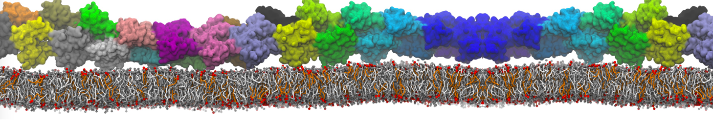
How to set-up a protein simulation?

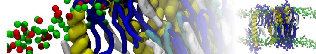
Keeping in line with the overall MARTINI philosophy, the coarse-grained protein model groups ∼4 heavy atoms together in one CG bead. Each residue has one backbone bead and zero or more side-chain beads depending on the amino acid type. The secondary structure of the protein influences both the selected bead types and bond/angle/dihedral parameters of each residue as explained in Monticelli et al. (J Comput Chem Theory, 2008). It is noteworthy that, even though the protein is free to change its tertiary arrangement, local secondary structure is pre-defined and thus static throughout a simulation. Conformational changes that involve changes in the secondary structure are therefore beyond the scope of Martini CG proteins.

Setting up a CG protein simulation consists basically of two steps: 1) converting an atomistic protein structure into a CG model and 2) generating a suitable Martini topology. Both these steps are easy to do with the martinize.py script

How do I model DNA and other nucleotides?

We are in the process to develop an extension of Martini toward nucleotides. A beta version is now available!

How do I use the polarizable water model and when should I use it?

How? Easy, use the special martini_v2.P.itp file in which the polarizable water model is defined - it also contains the full interaction matrix with all other particles. You can combine it with any other topology file, either 2.0 or 2.1. Only in the latter case please note that particle types AC1 and AC2, used for certain apolar amino acids, are obsolete and should be replaced by norma C1 and C2 particle types. Furthermore, don't forget to set the relative dielectric screening to eps=2.5 instead of eps=15 in standard Martini. See the example mdp file, have a look at the example applications featuring a box of pure polarizable water, and check out the script to convert standard water into polarizable water. And last, please have a look at the paper describing the polarizable model:

[1] S.O. Yesylevskyy, L.V. Schafer, D. Sengupta, S.J. Marrink. Polarizable water model for the coarse-grained Martini force field. PLoS Comp. Biol, 6:e1000810, 2010. open access.

When? We first note that the polarizable Martini water model is not meant to replace the standard Martini water model, but should be viewed as an alternative with improved properties in some, but similar behaviour at reduced efficiency in other applications. It is 2 to 3 times more expensive than standard Martini because the polarizable water bead has three particles. In combination with PME, which you can do with the polairzable model, it is even slower. However, for systems or processes in which charges or polar particles are present in a low-dielectric medium (e.g., inside a bilayer, or protein), the polarizable water model is much more realistic as it captures the dielectric inhomogeneity of the system. Furthermore, the effect of electrostatic fields (both external and internal) is modeled more realistically. In fact you may even simulate cool phenomena like electroporation.